SES Toolbox webpage
Home FAQ Download Discussion group Contact
us
You can also download the offline pdf version of this FAQ.
Section 1 - General Information
Section 2 - Installation
Section 3 - Getting started
What is SES Toolbox made for?
What is a point process?
What is a similarity measure?
What
is a spike train?
What is a Morris-Lecar
neuron?
What is EEG?
What
are steady-state visually evoked potentials?
What are auditory evoked potentials (AEP)?
What is a time-frequency map?
What is a bump?
What is Hilbert-Huang transform?
What is empirical mode
decomposition?
What is cell migration?
The SES Toolbox contains Matlab
scripts for computing SES similarity measures. SES stands for Stochastic
Event Synchrony, and is a family of similarity measure
for point processes.
SES can be applied to one-dimensional (e.g., spike trains) and
multi-dimensional point processes (e.g., sparse time-frequency
representations of electrophysiological signals such as matching-pursuit
representations, chirplets,
Hilbert-Huang
transforms, and bump
models).
SES tries to align
events in the point processes; the better the alignment, the more similar the point
processes are considered to be. More precisely, the similarity is quantified by
the following parameters: time delay, variance of the timing jitter, fraction
of "non-aligned'' events, and average similarity of the aligned events.
The SES measures may be viewed as
extensions of the cost-based
metrics of Victor et al. SES gives a statistical interpretation of those
metrics, and therefore, it is able to automatically infer the unit costs, in
contrast to the cost-based metrics. The latter are so far only applicable to
one-dimensional point processes, whereas SES is applicable to multi-dimensional
point processes as well.
We have used SES to:
·
quantify
the firing reliability of Morris-Lecar neurons,
·
detect
loss of EEG synchrony in Mild
Cognitive Impairment patients,
·
analyze
steady-state visually evoked potentials and EEG
responses to auditory stimuli,
·
investigate
the causal relation between morphological and molecular signaling events in cell migration.
In mathematics, a point
process is a random element whose values are "point patterns"
on a set S. While in the exact mathematical
definition a point pattern is specified as a locally finite counting measure, it is sufficient for more applied
purposes to think of a point pattern as a countable
subset of S that has no limit
points.
Point processes are well studied
objects in probability theory
and a powerful tool in statistics for modeling and analyzing spatial data,
which is of interest in such diverse disciplines as forestry, plant ecology,
epidemiology, geography, seismology, materials science, astronomy, and others.
Point processes on the real line form an important special case that is
particularly amenable to study,
because the different points are ordered in a natural way, and the whole point
process can be described completely by the (random) intervals between the
points. These point processes are frequently used as models for random events
in time, such as the arrival of customers in a queue (queueing
theory), of impulses in a neuron, referred to as "spike trains" (computational neuroscience), particles
in a Geiger counter, or of searches on the world-wide
web.
Source: http://en.wikipedia.org/wiki/Point_process
SES (Stochastic Event Synchrony)
is a family of similarity measures for point
processes. It may be applied to one-dimensional and multi-dimensional point
processes.
Similarity is some degree of symmetry in
either analogy
and resemblance
between two or more concepts or objects.
The notion of similarity rests either on exact or approximate repetitions of patterns in the compared
items. In the case of approximate repetitions we talk about statistical
similarity as found in a fractal and its parts. Finding similarities or distinguishing
between dissimilarities depends on the faculties of pattern recognition and disambiguation,
respectively.
Source: http://en.wikipedia.org/wiki/Similarity
A similarity measure is a
function that associates a numeric value with sequences such that a higher
value indicates greater similarity.
SES (Stochastic Event Synchrony)
is a family of similarity measures for point
processes. It may be applied to one-dimensional and multi-dimensional point processes.
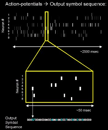
Neurons are remarkable among the cells
(biology) of the body in their ability to propagate signals rapidly over
large distances. They do this by generating characteristic electrical pulses
called action potentials or, more simply, spikes
that can travel down nerve fibers. Sensory neurons change their activities by
firing sequences of action potentials in various temporal patterns, with the
presence of external sensory stimuli, such as light, sound, taste, smell and touch. It is known
that information about the stimulus is encoded in this pattern of action
potentials and transmitted into and around the brain. It is also discovered
that muscles
are activated by action potentials and that motor
neurons serve to convert action potentials generated by the brain into
muscle movements that allow animals to interact with the environment, often in
response to sensory stimuli they receive from it.
Although action potentials can
vary somewhat in duration, amplitude and shape, they are typically treated as identical stereotyped
events in neural coding studies. If the brief duration of an action potential
(about 1ms) is ignored, an action potential sequence, or spike train,
can be characterized simply by a series of all-or-none point events in time.
Sources: http://en.wikipedia.org/wiki/Neural_encoding and www.kyb.tuebingen.mpg.de
We have applied SES to spike trains generated by Morris-Lecar neurons, with the aim of quantifying the
firing reliability of those neurons.
What is a Morris-Lecar neuron?
The Morris-Lecar
neuron model is two-dimensional "reduced" dynamical model for the
membrane potential of a neuron;
it exhibits properties of type I and II neurons [Gutkin
and Ermentrout].
The spiking behavior differs in both neuron types. To illustrate this, we show
the membrane potential for 5 trials (left: type I neuron; right: type II
neuron), where the input current consists of a baseline, a sinusoidal
component, and additive Gaussian noise [Robinson,
Dauwels et al.]:
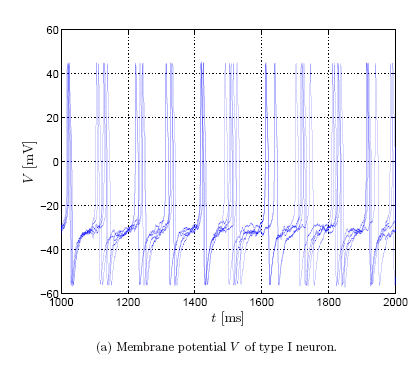
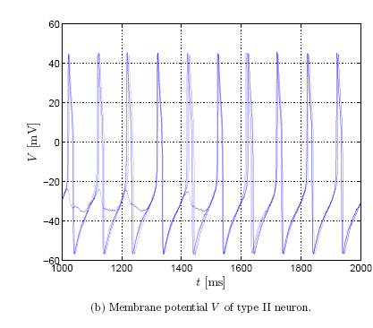
The sinusoidal component forces
the neuron to spikes regularly, however, the precise timing varies from trial
to trial due to the additive Gaussian noise.
This can be seen more clearly from the corresponding rasterplots (50 trials),
obtained by thresholding the membrane potential:
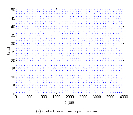
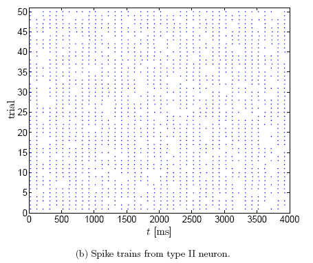
In type II neurons, the timing jitter is small, but spikes tend to drop out. In
type I neurons, on the other hand, fewer spikes drop out, but the dispersion of
spike times is larger. In other words, type II neurons prefer to stay coherent
or to be silent, on the other hand, type I neurons follow the middle course
between those two extremes [Robinson].
This difference in spiking
behavior is due to the way periodic firing is established. In type I neurons,
periodic firing results from a saddle-node bifurcation of equilibrium points.
Such neurons show a continuous transition from zero frequency to arbitrary low
frequency of firing. Pyramidal cells are believed to be type I neurons. On the
other hand, in type II neurons, periodic firing occurs by a sub-critical
Hopf-bifurcation. Such neurons show an abrupt onset of repetitive firing at a
higher firing frequency, they cannot support regular low-frequency firing.
Squid giant axons and the Hodgkin-Huxley model are type II [Gutkin and Ermentrout, Robinson].
For
more detailed information on Morris-Lecar neurons, click here.
References:
·
B. S.
Gutkin and G. B. Ermentrout,
Dynamics of membrane excitability determine interspike interval variability: a
link between spike generation mechanisms and cortical spike train statistics.
Neural Computation 10, 1047–1065, 1998.
·
H. P.
C. Robinson,
The biophysical basis of firing variability in cortical neurons,
Chapter 6 in Computational Neuroscience: A Comprehensive Approach, Mathematical
Biology & Medicine Series, Edited By Jianfeng Feng, Chapman & Hall/CRC,
2003.
·
J.
Dauwels, F. Vialatte, T.Weber, and A. Cichocki,
Quantifying Statistical Interdependence by Message Passing on Graphs PART I:
One-Dimensional Point Processes, Neural Computation,
PDF file, 1512 KB.
In the last paper in the above list, we apply SES to spike trains generated by Morris-Lecar neurons (type I and II), with the
aim of quantifying the firing reliability of those neurons.
We observed that the event reliability is significantly smaller in type
I than in type II neurons, in contrast, the timing dispersion is
vastly larger.
This agrees with our intuition: since in type II neurons spikes tend to drop
out, the event reliability should be larger. On the other hand, since the
timing dispersion of the spikes in type I is larger, we expect the timing
dispersion to be larger in those neurons.
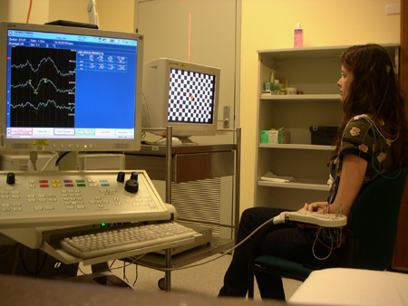
Electroencephalography (EEG), in the broadest sense of the term,
refers to the measurement of the electrical
activity produced by the brain. In clinical contexts, EEG refers to the recording of the
brain's spontaneous electrical activity in the time-domain
as recorded from multiple electrodes placed on the scalp. In neurology, the
main diagnostic
application of EEG is in the case of epilepsy, as
epileptic activity can create clear abnormalities on a standard EEG study. A
secondary clinical use of EEG is in the diagnosis of coma and encephalopathies.
EEG used to be a first-line method for the diagnosis of tumors, stroke and other
focal brain disorders, but this use has decreased with the advent of anatomical
imaging modalities, such as MRI and CT.
Derivatives of the EEG technique
include evoked potentials (EP), which involves averaging
the EEG activity time-locked to the presentation of a stimulus of some sort
(visual, somatosensory, or auditory). Event-related potentials refer to averaged
EEG responses that are time-locked to more complex processing of stimuli; this
technique is used in cognitive science, cognitive psychology, and psychophysiological
research.

Sources:
http://en.wikipedia.org/wiki/Electroencephalography
and http://www.drzekin.hit.bg
We have applied SES to the EEG of Mild
Cognitive Impairment patients, under resting conditions:
·
J.
Dauwels, F. Vialatte, T.Weber, T. Musha and A. Cichocki,
Quantifying Statistical Interdependence by Message Passing on Graphs PART II:
Multi-Dimensional Point Processes, Neural Computation.
PDF file, 857 KB.
·
J.
Dauwels, T. Weber, F. Vialatte, and A. Cichocki,
Quantifying the Similarity of Multiple Multi-Dimensional Point Processes by
Integer Programming with Application to Early Diagnosis of Alzheimer’s Disease
from EEG,
Proc. 30th Annual International Conference of the IEEE Engineering in Medicine
and Biology Society (EMBC08).
PDF file, 219 KB.
·
J.
Dauwels, F. Vialatte, M. Vialatte, and A. Cichocki,
A Comparative Study of Synchrony Measures for the Early Diagnosis of
Alzheimer’s Disease Based on EEG, NeuroImage, under revision.
We also have analyzed the EEG responses to visual
and auditory stimuli, using SES.
What are
steady-state visually evoked potentials?
Steady State Visually Evoked
Potentials (SSVEP) are
signals that are natural responses to visual stimulation
at specific frequencies.
When the retina
is excited by a visual stimulus ranging from 3.5 Hz to 75 Hz, the brain
generates electrical activity at the same (or multiples of) frequency of the
visual stimulus.
This technique is used widely
with electroencephalographic
research regarding vision. SSVEP's are useful in research because of the
excellent signal-to-noise ratio and relative immunity to
artifacts. SSVEP's also provide a means to characterize preferred frequencies
of neocortical dynamic processes. SSVEP is generated by stationary localized
sources and distributed sources that exhibit characteristics of wave phenomena.
Sources: http://en.wikipedia.org/wiki/Steady_state_visually_evoked_potential
and www.virtualmedicalcentre.com
We have analyzed Steady State Visually Evoked Potentials, using SES:
·
J.
Dauwels, T. Rutkowski, F. Vialatte, and A. Cichocki,
On the Synchrony of Empirical Mode Decompositions with Application to EEG,
Proc. IEEE Int. Conf. on Acoustics and Signal Processing (ICASSP), 2008.
·
F.
Vialatte, J. Dauwels, T. Rutkowski, and A. Cichocki,
Oscillatory Event Synchrony during Steady State Visually Evoked Potentials,
Advances in Cognitive Neurodynamics, Springer, October 2008.
·
F.
Vialatte, J. Dauwels, M. Maurice, and A. Cichocki,
Steady-state visually evoked potentials: time-frequency analysis and
oscillatory event synchrony, submitted to Cognitive Neurodynamics.
What are auditory evoked potentials?
Auditory
evoked potential can be used to trace the signal generated by a sound, from the
cochlear
nerve, through the lateral lemniscus, to the medial geniculate nucleus, and to the cortex.

Auditory evoked potentials (AEPs)
are a subclass of event-related potentials (ERP)s. ERPs are brain responses
that are time-locked to some “event”, such as a sensory stimulus, a mental
event (such as recognition of a target stimulus), or the omission of a
stimulus. For AEPs, the “event” is a sound. AEPs (and ERPs) are very small
electrical voltage potentials originating from the brain recorded from the
scalp in response to an auditory stimulus, such as different tones, speech
sounds, etc.
Source: http://en.wikipedia.org/wiki/Evoked_potential#Auditory_evoked_potential
and http://www.iurc.montp.inserm.fr
We have analyzed auditory evoked potentials, using SES:
·
T.
Rutkowski, J. Dauwels, F. Vialatte, and A. Cichocki,
Time-Frequency and Synchrony Analysis of Responses to Steady-state Auditory and
Musical Stimuli from Multichannel EEG,
NIPS Workshop on Music, Brain and Cognition, 2007.
PDF file, 173 KB.
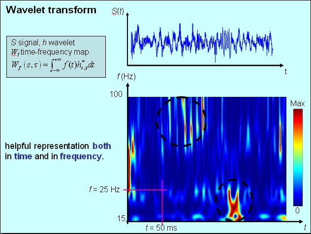
A time-frequency map conveniently
represents simultaneously time and frequency information. The Fourier spectrum
of a signal represents the frequency content of the signal, the signal itself is
in the time domain. In time-frequency maps, the frequency spectum is given for
each time step so that one can see the evolution of the frequencies.
Time-frequency maps can for example be computed using windowed multitaper methods or wavelets.
We have applied SES to sparse time-frequency
representations (Morlet wavelets)
of EEG signals, referred to as "bump
models":
·
J.
Dauwels, F. Vialatte, T.Weber, T. Musha and A. Cichocki,
Quantifying Statistical Interdependence by Message Passing on Graphs PART II:
Multi-Dimensional Point Processes, Neural Computation.
PDF file, 857 KB.
·
J.
Dauwels, T. Weber, F. Vialatte, and A. Cichocki,
Quantifying the Similarity of Multiple Multi-Dimensional Point Processes by
Integer Programming with Application to Early Diagnosis of Alzheimer’s Disease
from EEG,
Proc. 30th Annual International Conference of the IEEE Engineering in Medicine
and Biology Society (EMBC08).
PDF file, 219 KB.
·
J.
Dauwels, F. Vialatte, M. Vialatte, and A. Cichocki,
A Comparative Study of Synchrony Measures for the Early Diagnosis of
Alzheimer’s Disease Based on EEG, NeuroImage, under revision.
In our context, we loosely
define a bump as a parametric function used for atomic decomposition of the time-frequency map. Usually, half-ellipsoid bumps are
used. See Vialatte et al. 2007 and bump toolbox website.

We have applied SES to bump
models of EEG signals:
·
J.
Dauwels, F. Vialatte, T.Weber, T. Musha and A. Cichocki,
Quantifying Statistical Interdependence by Message Passing on Graphs PART II:
Multi-Dimensional Point Processes, Neural Computation.
PDF file, 857 KB.
·
J.
Dauwels, T. Weber, F. Vialatte, and A. Cichocki,
Quantifying the Similarity of Multiple Multi-Dimensional Point Processes by
Integer Programming with Application to Early Diagnosis of Alzheimer’s Disease
from EEG,
Proc. 30th Annual International Conference of the IEEE Engineering in Medicine
and Biology Society (EMBC08).
PDF file, 219 KB.
·
J.
Dauwels, F. Vialatte, M. Vialatte, and A. Cichocki,
A Comparative Study of Synchrony Measures for the Early Diagnosis of Alzheimer’s
Disease Based on EEG, NeuroImage, under revision.
What is Hilbert-Huang transform?
The Hilbert-Huang Transform
(HHT) is a way to decompose a signal
into so-called intrinsic mode functions (IMF), and obtain instantaneous frequency data. It is
designed to work well for data that are nonstationary and nonlinear. In
contrast to other common transforms like the Fourier
Transform, the HHT is more like an algorithm (an empirical approach) that
can be applied to a data set, rather than a theoretical tool. Almost all the case
studies reveal that the HHT gives results much sharper than any of the
traditional analysis methods in time-frequency-energy representation.
Additionally, it reveals true physical meanings in many of the data examined.
The Hilbert-Huang transform
(HHT) is the result of the empirical mode decomposition (EMD) and the Hilbert spectral analysis (HSA). The HHT
uses the EMD method to decompose a signal
into so-called intrinsic mode function, and uses the HSA method to obtain instantaneous frequency data. The HHT
provides a new method of analyzing nonstationary and nonlinear time
series data.
The fundamental part of the HHT
is the empirical mode decomposition (EMD) method. Using the EMD
method, any complicated data set can be decomposed into a finite and often
small number of components, which is a collection of intrinsic mode
functions (IMF). An IMF represents a generally simple oscillatory
mode as a counterpart to the simple harmonic function.
By definition, an IMF is any function with the same number of extrema
and zero crossings, with its envelopes being symmetric with respect to zero.
The definition of an IMF guarantees a well-behaved Hilbert
transform of the IMF. This decomposition method operating in the time
domain is adaptive and highly efficient. Since the
decomposition is based on the local characteristic time scale of the data, it
can be applied to nonlinear and nonstationary processes.
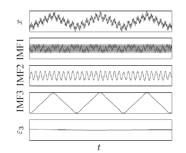
Three IMFs extracted from a given signal (top);
also shown is the residue (bottom)
The Hilbert spectral analysis (HSA) provides
a method for examining the IMF's instantaneous frequency data as functions
of time that give sharp identifications of imbedded structures. The final presentation
of the results is an energy-frequency-time distribution, designated as the Hilbert
spectrum.
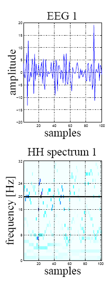
The HHS (bottom) of a 20Hz SSVEP signal
(top).
Source: http://en.wikipedia.org/wiki/Hilbert-Huang_Transform
We have used SES to analyze the synchrony of Hilbert-Huang
transforms:
·
T.
Rutkowski, J. Dauwels, F. Vialatte, and A. Cichocki,
Time-Frequency and Synchrony Analysis of Responses to Steady-state Auditory and
Musical Stimuli from Multichannel EEG,
NIPS Workshop on Music, Brain and Cognition, 2007.
PDF file, 173 KB.
·
J.
Dauwels, T. Rutkowski, F. Vialatte, and A. Cichocki,
On the Synchrony of Empirical Mode Decompositions with Application to EEG,
Proc. IEEE Int. Conf. on Acoustics and Signal Processing (ICASSP), 2008.
What is empirical mode decomposition?
Cell migration is a central process in the development
and maintenance of multicellular organisms. Tissue formation
during embryonic development, wound
healing and immune responses all require the orchestrated
movement of cells in a particular direction to a specific location. Errors
during this process have serious consequences, including mental retardation, vascular disease, tumor formation and metastasis.
An understanding of the mechanism by which cells migrate may lead to the
development of novel therapeutic strategies for controlling , for example,
invasive tumour cells. Cells in animal tissues often migrate in response to,
and towards, specific external signals, a process called chemotaxis.

Source: http://en.wikipedia.org/wiki/Cell_migration
and http://ocw.mit.edu
Using SES, we investigated some aspects of
the dynamics of cell migration. More specifically, we analyzed time-lapse fluorescence
resonance energy transfer (FRET) images of Rac1 in motile HT1080 cells, which are human fibrosarcoma cells [Dauwels et al.]. The protein Rac1 is well known to induce
filamentous structures that enable cells to migrate. We analyzed the
statistical relation between Rac1 activity events and morphological events. For
this purpose, we developed a novel computational method for quantifying those
interdependencies. This method consists of two steps:
·
We
first determine the morphological and molecular activity events from the
time-lapse microscopy images. To this end, we apply edge evolution tracking
(EET) [Tsukada et al.]: it
identifies cellular-morphological events and molecular-activity events, and
determines the distance in space between those events, taking the evolution of
the cell morphology into account.
·
Next
we quantify the interdependence between those morphological and activity events
by means of SES: using the EET
distance measure [Tsukada
et al.], SES tries to align cellular morphological with molecular
activity events; the better this alignment can be carried out, the more similar
the event sequences are considered to be. In addition, the method is able to
determine delays between both event sequences.
We found that the delay between
morphological events and activity events is negative; in other words, on
average the morphological events occur first, followed by activity events: first
the cell expands, then there is an influx of Rac1.
References:
·
J.
Dauwels, Y. Tsukada, Y. Sakumura, S. Ishii, F. Vialatte, and A. Cichocki,
On the synchrony of morphological and molecular signaling events in cell
migration,
International Conference on Neural Information Processing, November 25–28,
2008, Auckland, New Zealand 2008.
PDF file, 506
KB.
·
Tsukada,
Y., Aoki, K., Nakamura, T., Sakumura, Y., Matsuda, M., and Ishii, S.
Quantification of local morphodynamics and local GTPase activity by edge
evolution tracking
PLoS
Computational Biology 4(11): e1000223. doi:10.1371/journal.pcbi.1000223
Downloading the toolbox
Installing the packages
Go to the [Download] section.
Click on the links and save the
file on your local hard disk. Unzip the zip file.
If you do not have Winzip or similar software, click here to download the latest Winzip.
The "Toolbox"
directory contains the core m-files of the toolbox. That directory is
further divided into the directories "Pair_one_dim" and "Pair_multi_dim",
which contain scripts of the SES measures for pairs of one-dimensional and
multi-dimensional point processes respectively.
The "Demo"
directory contains sample m-files used to run the toolbox. It is also divided
into the directories "Pair_one_dim" and "Pair_multi_dim",
which contain demos for one-dimensional and multi-dimensional point processes
respectively.
In later versions, we will
also include SES measures for collections of one-dimensional or
multi-dimensional point processes.
xxxxxxxxxxxxxxxxxxxxxxxxx
How must I proceed to do an experiment with the
toolbox?
How can I use my own signals with the toolbox?
How must I proceed to do
an experiment with the toolbox?
xxxxxxxxxxxxxxxxxxxxxxxxx
How can I use my own signals with the toolbox?
xxxxxxxxxxxxxxxxxxxxxxxxx